Introduction
This blog post introduces a new custom study to Sierra Chart which adds two popular risk metrics: value at risk (VaR) and conditional value at risk (CVaR). The study does a historical VaR and CVaR calculation given the length of the look back period and the confidence interval.
If you are unfamiliar with what VaR or CVaR are, I will briefly describe them in the next section. If you are already familiar what these metrics are, feel free to skip to next section.
An Introduction to VaR and CVaR
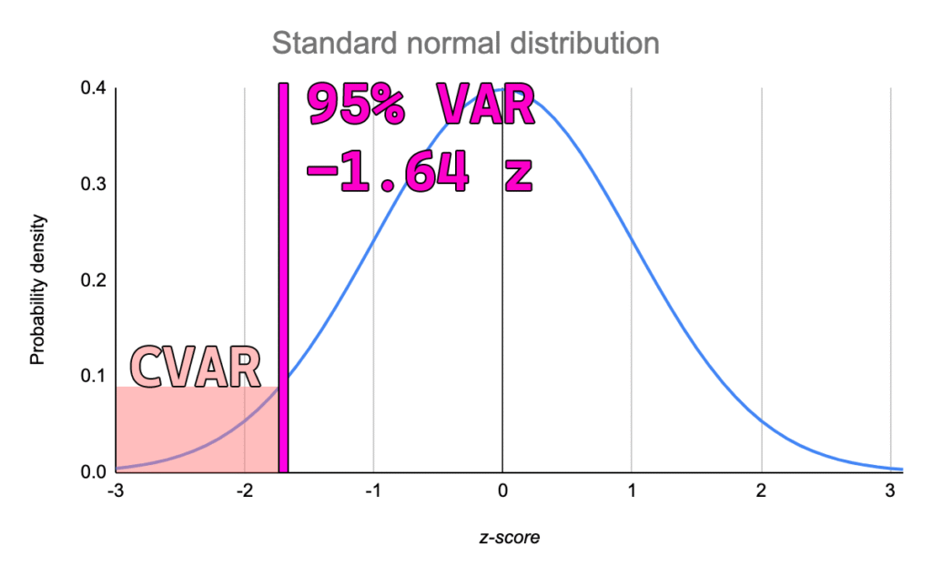
VaR and CVaR are two common risk measures that help describe the distribution of losses from an asset or portfolio. Both measures require 2 inputs; the look back period (x) and the confidence interval (y).
“VaR is the loss level we do not expected to be exceeded over the time horizon at the specified confidence interval” – GARP (2022)
There are multiple different ways to calculate VaR such as historical simulation or monte carlo simulation. Historical simulation is done by sorting previous returns over period x and choosing the yth percentile return for VaR. CVaR is then the average of the remaining realizations that exceed the VaR level.
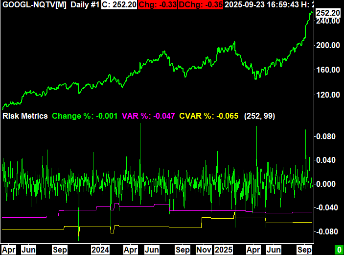
Study Settings
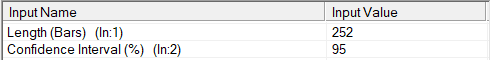
The study comes with a total of 5 sub graphs and 2 inputs.
Inputs
- Length (Bars): The look back period in chart bars
- Confidence Interval (%): The confidence interval to run the analysis with
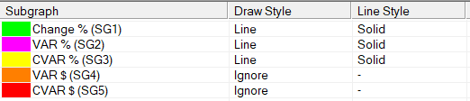
Subgraphs
- Change %: Percent change from today’s last price from yesterday’s last price
- VAR %: The value at risk shown as a percentage
- CVAR %: The conditional value at risk shown as a percentage
- VAR $: The value at risk shown in dollars (VAR% * Last Price)
- CVAR $: The conditional value at risk shown in dollars (CVAR% * Last Price)
Interpretation
VaR and CVaR ultimately exist to represent the risk of the specific asset that is being charted. Therefore, the most elementary interpretation is that the more negative the numbers, the higher the risk you should expect.
Many investors might choose to look at standard deviation of returns or the price of an asset as the “risk,” but VaR and CVaR are often better representations. Furthermore, if given two identical investments with identical VaR but one has a higher CVaR, the one with the higher CVaR is considered riskier. This is because the larger CVaR means that when losses do exceed the VaR, they are larger in magnitude.
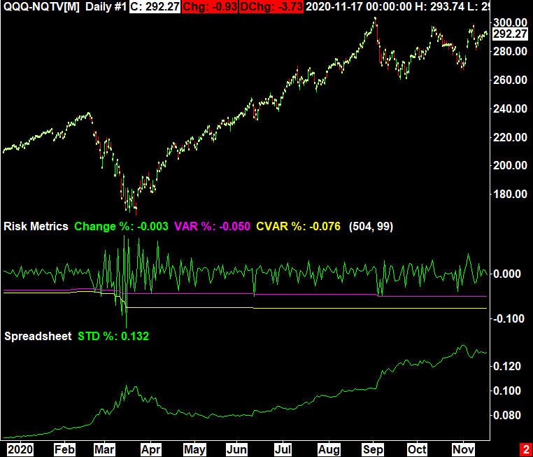
The image to the right shows the difference between VaR calculations and the standard deviation of returns during the COVID-19 pandemic using a 2 year look back period. VaR is more responsive and gives investors a more logical way to think about risk than simply standard deviation of returns.
Implementation
The implementation of a historical VaR analysis is relatively simple and involves 2 main steps. The first step is to accumulate and sort the previous percent changes into an array. The next step is to calculate which item in the array corresponds with the given confidence interval.
The code block to the right shows the implementation used in the study.
One traditional feature of VaR that this implementation does not include is interpolation between data points. For example, in traditional VaR if there is a look back period of 150 with 99% confidence, the VaR will be the average between the 2nd and 3rd largest losses. In my implementation, the VaR is rounded to the nearest real occurrence (variable name VARIndex). This will produce minor difference in the calculation compared to interpolation, but these differences do not dramatically impact the interpret-ability or usefulness of the indicator. Furthermore, if you are using a look back period that evenly divides by (1-Confidence Interval), there is not interpolation required and therefore the answer is exact.
struct RiskMetrics
{
	float VAR = 0.0f;
	float ES = 0.0f;
};

RiskMetrics GetRiskMetrics(SCStudyGraphRef sc, SCSubgraphRef PercentChanges, int Length, float Percentile)
{
	RiskMetrics rm;

	if (Percentile > 100.0f) return rm;

	std::vector<float> Changes;
	Changes.reserve(Length);

	for (int i = sc.Index; i > sc.Index - Length; i--)
		Changes.push_back(PercentChanges[i]);

	std::sort(Changes.begin(), Changes.end());

	if (Percentile == 100.0f)
	{
		rm.VAR = Changes[0];
		rm.ES = Changes[0];
		return rm;
	}

	float ItemWidth = 100.0f / static_cast<float>(Changes.size());

	float Intermediate = (100.0f - Percentile) / ItemWidth;

	uint32_t VARIndex = std::round(Intermediate);

	rm.VAR = Changes[VARIndex];

	for(int i = 0; i < VARIndex; i++)
		rm.ES += Changes[i];

	rm.ES /= static_cast<float>(VARIndex);

	return rm;
}